how to make a scatter plot in Excel
Scatter plots are excellent charts for showing a relationship between two numerical variables across a number of unique observations. We see them in business communications from time to time, although they’re much more commonly used in the “exploration” part of the process—when we’re still trying to understand our data and find the important insights.
If you’re unfamiliar with scatter plots, their common use cases, or their benefits and drawbacks in a range of scenarios, check out the what is a scatter plot? article in our SWD Chart Guide. There, we explore some of the basics of scatter plots via an example, share tips for designing them more effectively, and discuss common variations (bubble charts, connected scatter plots, and more).
In this article we’ll walk through the steps of creating a scatter plot in Microsoft Excel. We’ll use a small dataset to:
create a simple scatter plot with a single data series;
modify that graph to show multiple data series in one scatter plot;
learn how to add contextual elements to our view (like averages, quadrant lines, and trendlines);
add data labels to all, or just a few, points in our graph; and
create custom labels using other fields in our dataset.
The scenario
Four years ago, our organization wanted to find a way to make newly-hired junior analysts more successful and effective. We launched a small, competitive pilot program that would start new employees with a full year of dedicated and comprehensive training. All other junior hires would continue to receive the on-the-job, course-based and ad-hoc learning experience that we have traditionally provided.
We currently have 20 individuals who have completed the program. Each month, they and all the analysts in the organization have their performance rated as below-average, average, or above-average in comparison to their peers across our three global locations.
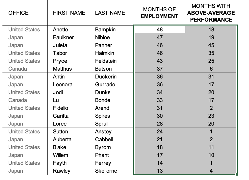
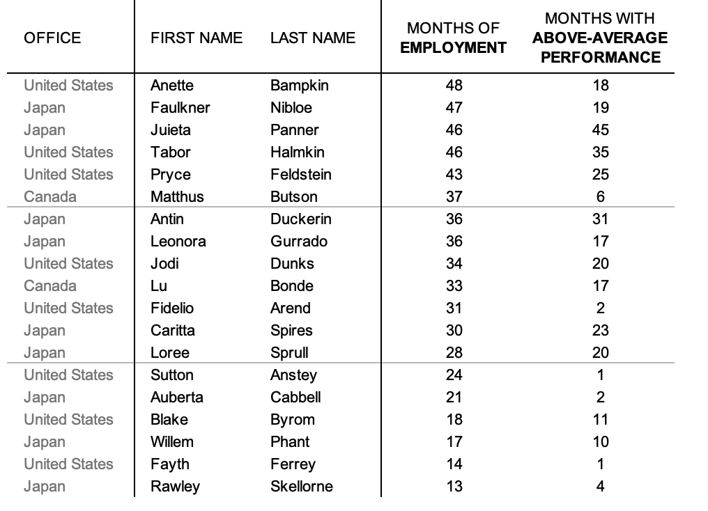
The following table shows our pilot program graduates, the number of months they’ve been with the organization, and how many months their performance has been rated “above average.”

This data table is the source for our scatter plot.
We’ll use this dataset to create and refine our scatter plots, reshaping it and adding to it as needed.
How to create a single-series scatter plot
The simplest way to create a scatter plot in Excel is to highlight the cells in the two columns that contain your two numeric variables—in this case, the “MONTHS OF EMPLOYMENT” and “MONTHS WITH ABOVE-AVERAGE PERFORMANCE” columns.
Highlight the two columns you want to include in your scatter plot.
Then, go to the “Insert” tab of your Excel menu bar and click on the scatter plot icon in the “Recommended Charts” area of your ribbon.
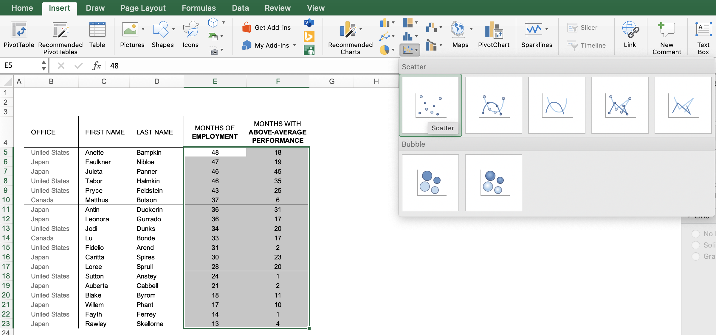
Select “Scatter” from the options in the “Recommended Charts” section of your ribbon.
Excel will automatically create a scatter plot for you in the same sheet as your data, using the first column of your dataset as the horizontal (X) axis, and the second column as your vertical (Y) axis.
A quick note here: in creating scatter plots, a common practice is to make the horizontal axis your “independent variable” and the vertical axis your “dependent variable” (that is, the number that is likely to change based on the value of our independent variable).
For our scenario, the number of months a person has been employed is more likely to affect the number of “above average” ratings they receive, rather than vice versa. That’s why our independent variable—months of employment—is in our data table’s left-hand column, and our dependent variable is in the right hand column.

Excel creates a scatter plot with these default settings.
This automatically-generated graph could use some formatting and cleanup. Taking time to strengthen the skeleton of your graph—everything that isn’t the actual data points—will help make your insights and information stand out.
After removing unnecessary lines, and cleaning up our axes and titles, our graph looks like this:
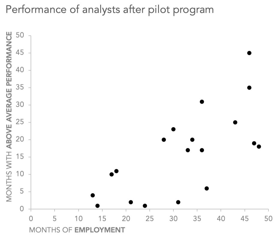
Now we have a nicely-formatted, single-series scatter plot that uses an identical black circle as a marker for each of our unique data points. From here, we can continue to make modifications and refinements to our graph.
How to create a scatter plot with multiple series
In the scatter plot we’ve just created, there is only one data series, consisting of our entire cadre of pilot program participants. Each participant’s length of employment is plotted on the horizontal axis, and their total of above-average monthly ratings is on the vertical axis.
Let’s assume we wanted to subdivide this data series into multiple series. For instance, our participants are assigned to three different offices worldwide (United States, Canada, and Japan); what if we wanted to color our data markers to represent that person’s location?
In Excel, creating a scatter plot with multiple data series can be done several ways. The easiest is to have a single column in your data containing the X values for all of your data series, and then have a separate column for the Y values of each individual data series.
Let’s take a look at how we could modify our existing data table to do this.
Our original data table, which we’ll modify in order to make a multi-series scatter plot.
In this table, the “OFFICE” is its own column, and it contains three unique values: United States; Japan; and Canada. Instead, add three new columns to the right of the existing table, and make each OFFICE value the name of one of the columns:
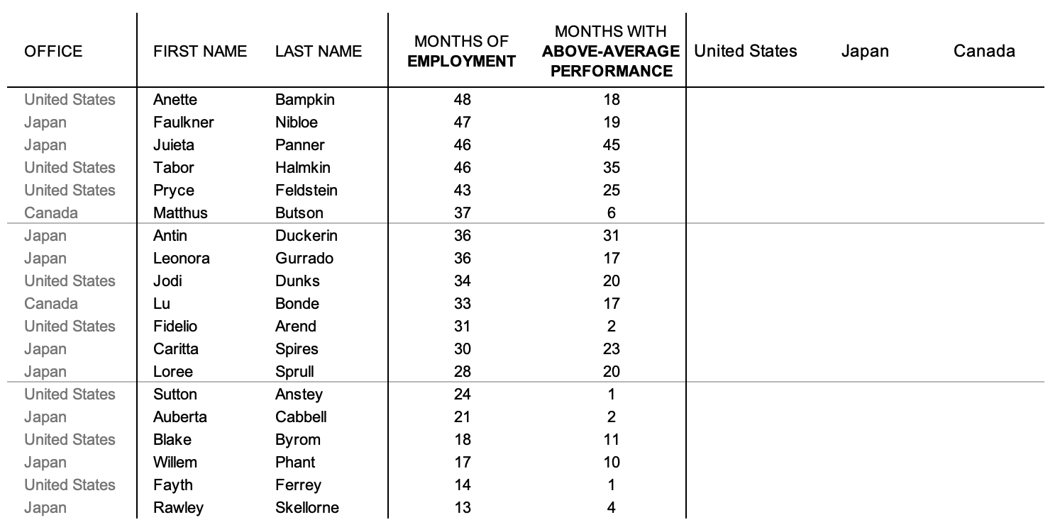
Add a column to the right for each of the three different offices.
In the cells of those columns, we’ll write a formula that says “If the value of [OFFICE] in this specific row matches the header of this column, then give this cell the same value as the [MONTHS WITH ABOVE AVERAGE PERFORMANCE] column; otherwise, give it a value of #N/A.”
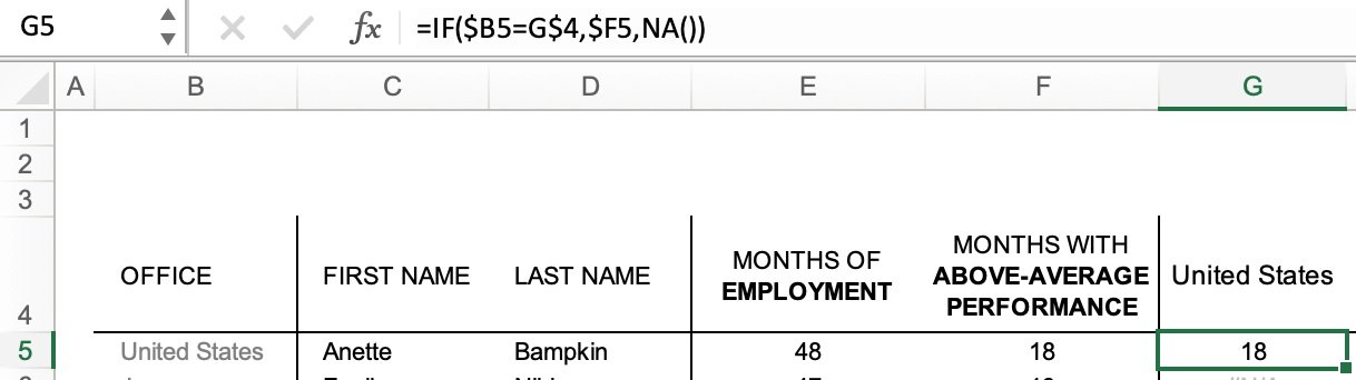
In cell G5, add a formula to decide if the cell should be empty, or should contain the value from cell F5.
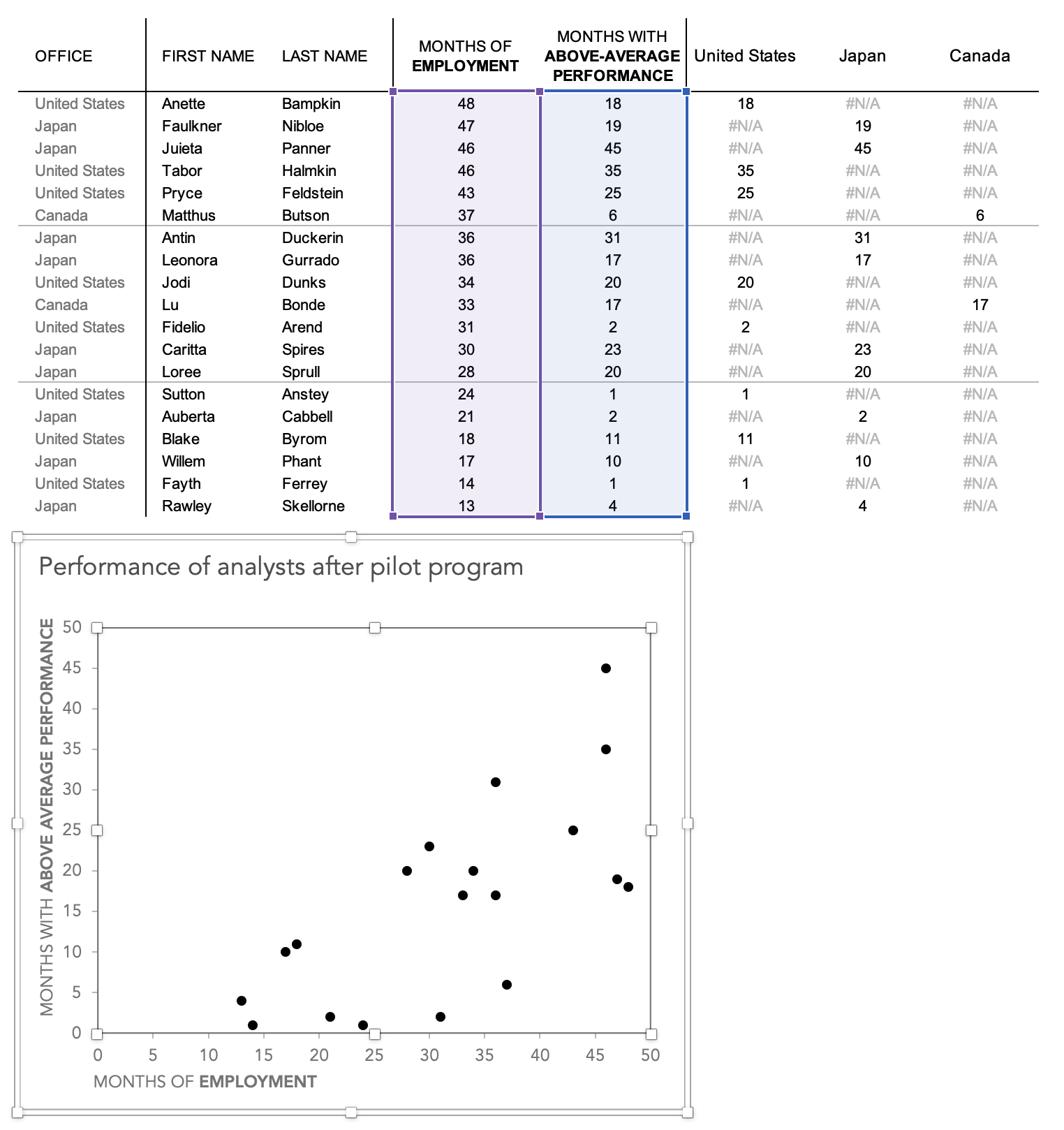
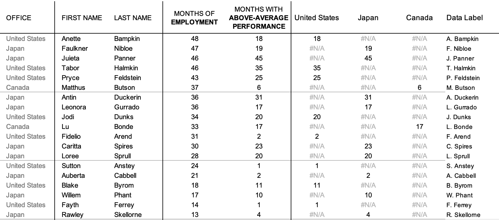
When we propagate this formula across our new columns and down all of our rows, the table will look like this:

Copy the Y values from column F into the appropriate column G, H, or I, based on if the OFFICE value in column A matches the header.
As you can see, our “United States” column only has numeric values if the “OFFICE” column value in that row is “United States.”
When you click on the existing scatter plot, you’ll see purple and blue highlighting around the X and Y columns that Excel is currently displaying in that graph.
Click on the scatter plot to highlight the columns Excel is using for the X (purple) and Y (blue) values.
We’d like this graph to show the Y values in the three new columns we’ve just created. To do that, hold your cursor over the edge of the blue rectangle until it becomes a hand, and then drag that rectangle right by a single column, so that it’s highlighting the data underneath “United States.”

Click and hold the blue column, and drag it to the right by a single column.
You might notice that a lot of your data points are now missing! That’s because now, Excel is only using the “United States” column for our Y axis, and Excel won’t draw a data point if there’s an “#N/A” as a Y value.
Not to worry, though: we’ll get all our data points back now, by clicking on the bottom right corner of that blue rectangle and dragging it to the right, so that the rectangle covers all three new columns we’ve created.

Click on the bottom right corner of the blue rectangle, and drag that corner to the right so that all three new columns are highlighted.
All of our data has returned, hooray! And, as you can see, Excel is now using a different color for each of our data series.
Let’s add a legend so that our viewers know what these different colors represent. First, we’ll name each of our data series: right-click on the chart, choose “Select Data,” and add the data series names manually in the pop-up window.

Type in the name of each series, or select a cell from the Excel sheet that contains the name.
Then, you can fine-tune the look of your graph—perhaps you add a legend as a subheader to your title, and pick specific colors for your series—and your multi-series scatter plot is ready to go.

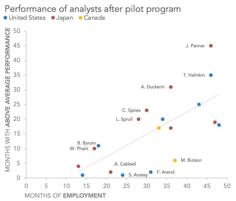
This scatter plot contains the same data as our first one, but the data is now subdivided into three series—one for each office—and is color-coded to reflect that. We’ve also added a legend beneath our chart title to identify which color goes with which office.
How to add averages, reference lines, and trendlines to a scatter plot
Whenever we present data to an audience who might be unfamiliar with it, it’s a good idea to include contextual information to help make it easier to understand. In a scatter plot, we can add context like:
What was the average X value?
What was the average Y value?
Was there a goal for either variable?
Is there a trend worth emphasizing?
Depending on the insights or the data itself, you might use one (or several) of these techniques, so let’s go through them one at a time.
How to add an average point to a scatter plot
We’ll start by adding another row to the bottom of our data table, where we’ll calculate what the average X and Y values were. For simplicity’s sake, we’re only going to look at the average across ALL of our participants, rather than separate averages for each office (although the same techniques would apply).
Since columns E and F contain our X and Y values, we’ll write formulas to average the values in each of those columns.
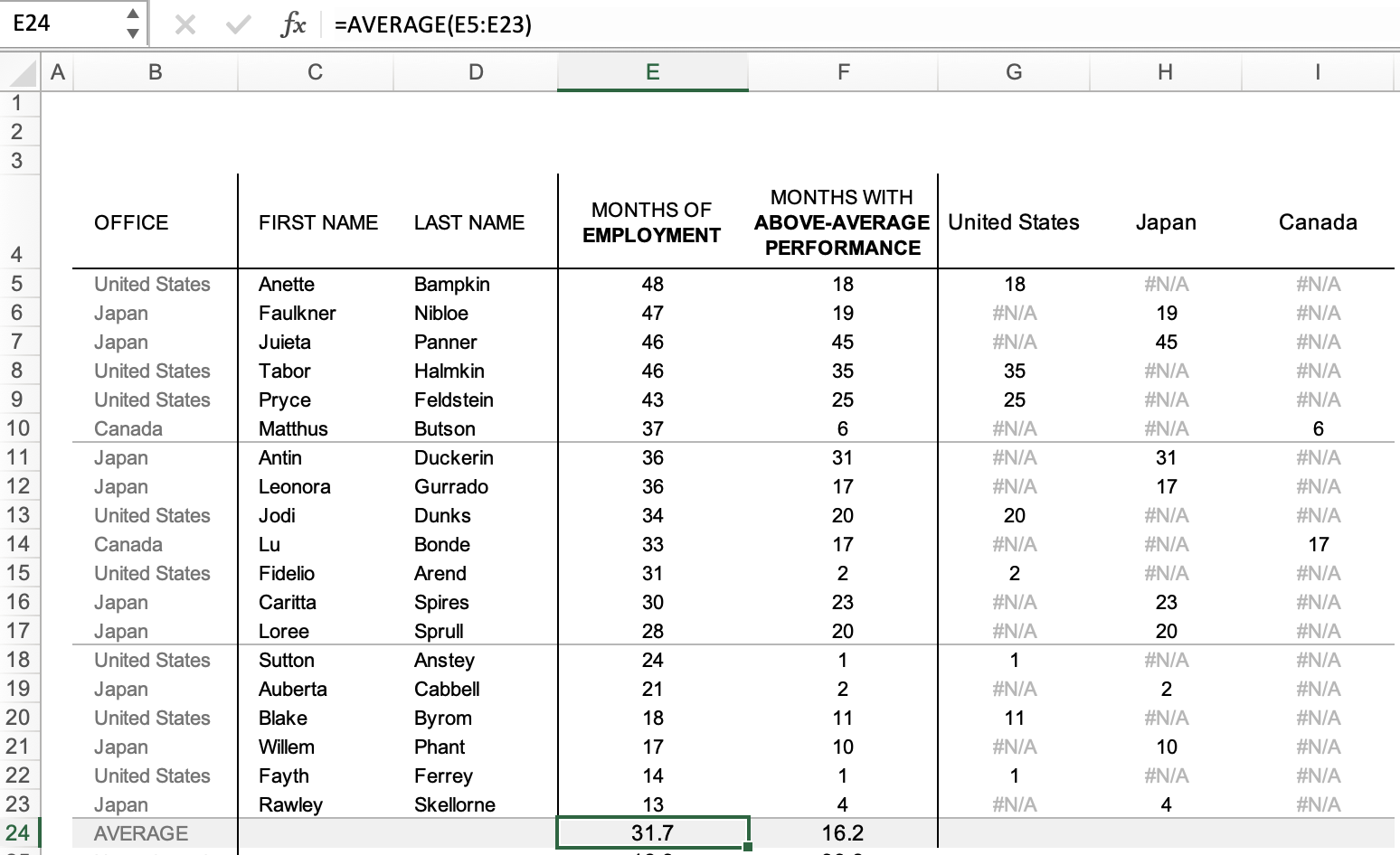
Row 24 will contain the averages of our X values (in column E) and our Y values (in column F). Use the AVERAGE formula, as shown in this screen capture, to generate the correct values.
Then, we’ll right-click on our chart, choose “Select Data…” from the menu that pops up, and add another data series just for our average values. Click the “+” button below the “Legend entries (Series):” window to add a new series, which you can then rename and set the range of X and Y values for in that pop-up.
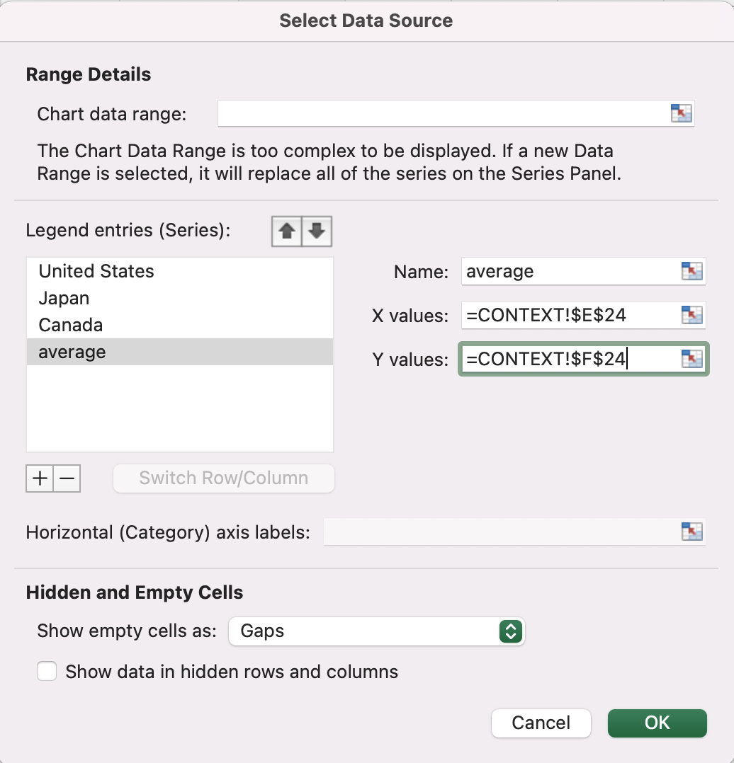
The “average” series will consist of a single point, showing the average of all X values and the average of all Y values.
That will put a single point on our chart that marks our X and Y averages, as you can see in the updated graph below.
I’ve deleted the new “average” series from the legend (by clicking once to highlight the legend, then a second time to highlight the average, and hitting “delete”), and formatted the single point to be gray with a black outline.

The average of X and Y values across all three data series is now shown in a single gray marker, outlined in black.
How to add reference lines and create quadrants in a scatter plot
Now that we have an average point, we can visually break our scatter plot into four quadrants:
above average in both X and Y variables;
below average in both;
high X but low Y; and
low X but high Y.
We’ll use our average point as the basis for drawing the lines that define those quadrants. Specifically, we’ll add a chart element to that point, and maybe not the one that you’d immediately expect: error bars.
Error bars are typically intended to show additional statistical context around a data point. Instead, we’ll be using them to draw both a vertical and a horizontal line, each of which will connect our axes to the edges of our graph, running directly through our average point.
First, we’ll need to know how long to make these error bars.
We know that each of our axes has a maximum value of 50, so we’ll make sure our error bars cover that total distance.
Vertically, we’ll draw one bar from the baseline to our average point, and one bar from our average point to the top of our graph.
Horizontally, we’ll draw one bar from our Y-axis to our average point, and then one bar from the average point to the right-hand edge of our graph.
To define the exact length of these error bar segments, we’ll add one more row of data to our table. Below the AVERAGE row, we’ll add a row called “Upper bound.” The value in those cells is calculated as “50-[average value]”.

Add an “Upper bound” row to the data set in preparation for building the quadrant lines.
Now, to add our error bars to the graph: click on the “average” data point in the chart, and then go to the Chart Design > Add Chart Element option in the ribbon, and select “Error Bars > More Error Bars Options...”
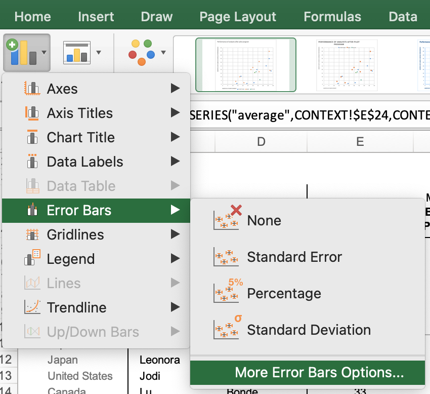
Here’s where to find the “More Error Bars Options” item in the drop-down menus.
This will open up a Format Error Bars pane on the right side of the screen. (At this point, Excel defaults to having you format the vertical error bars; we’ll get to the horizontal bars in a minute.) You’ll see options for “Direction” (select Both), “End Style” (select No Cap), and “Error Amount” (select Custom).

This screen shows the correct settings under “Format Error Bars.”
By selecting a Custom option under Error Amount, you’ll have to then click on the “Specify Value” button. In that popup window, tell Excel how far above and below your “average” point you want your vertical error bar to be drawn. That’s why we created that “upper bound” row of data earlier. For the “Positive Error Value” in the popup box, use the value from the “upper bound” row, and for the “Negative Error Value,” use the “AVERAGE” row value.

The vertical error bars are sized correctly, but the horizontal ones look like low-res wagon wheels. That’s what we’ll fix next.
Then, click directly on the horizontal error bars in the plot and follow the same steps to modify those bars, using the AVERAGE and Upper bound rows for the MONTHS OF EMPLOYMENT column.
(Note: these bars might be really small by default; if you can’t click on them, then click anywhere in your graph, then go to the “Format” menu next to “Chart Design”, and in the drop down menu on the far left of the ribbon, select “Series ‘average’ X Error Bars”.)

Quadrant lines are drawn, but could still use some re-formatting.
Once that’s done, you can modify the format of the lines and the average point however you like. I prefer to push these reference lines visually toward the background, and to make the average point itself invisible by turning off its data marker. (Careful! Don’t delete the data marker entirely, because that will also make the error bars disappear.)

With some formatting changes, our error bars have become perfectly sized quadrant lines, faded nicely into the background.
By drawing quadrants, I can see right away that we have two employees from the Japan office in the top left who have been above average on performance frequently, even though they’re among the newest 50% of program participants. Conversely, the yellow mark in the bottom right shows me that one participant has been here for a long time, but is far below the 50th percentile in terms of above-average performance periods. I don’t know if this is an interesting story, or the most important insight, but simply drawing the quadrants on the graph makes it easier for me to analyze, and talk about, some of the data points within it.
How to add trendlines to a scatter plot
Unlike drawing quadrant lines, drawing trendlines in Excel is fairly straightforward. Perhaps it’s TOO straightforward, actually; it’s awfully easy to put a trendline in a graph that doesn’t have any particular basis in reality, or doesn’t describe the actual trend in a way that would be useful for setting future expectations. Trendlines can also be attention-grabbing, adding visual clutter to a graph type that is already challenging for some viewers to accurately interpret. Typically, if there’s a trend worth highlighting, it’s already visible in the data without drawing an additional line on the graph itself.
Those concerns aside, a trendline can provide helpful context in certain situations. The graph we’re looking at, for instance, may benefit from some visual guidance showing us how well we should expect our pilot program cadre to perform, based on their experience at the company. A linear trendline could use historical data to provide some of that insight.
To create a trendline that uses all of our data points, we’ll create a fifth data series in addition to “United States,” “Canada,” “Japan,” and “average.” Right-click on the chart and choose “Select Data…”
In the popup window, add another data series that uses columns E and F (our original single-series data) as our X and Y values. I named it “for creating trendline.”
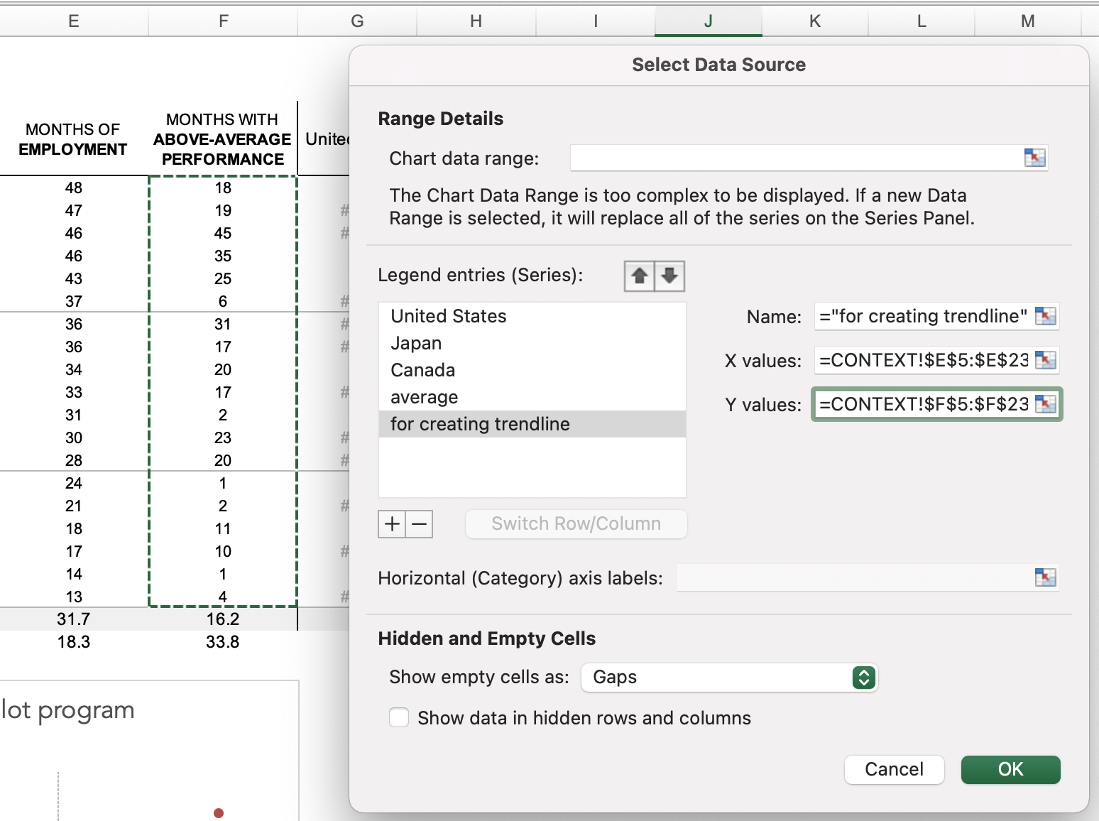
Add another data series to the view so that Excel can use it to calculate a trendline across all data points.
This data series will be plotted on top of all the existing series, using Excel’s default settings for size, color, and so on. In the view below, I’ve made the “for creating timeline” series markers larger and purple just so you can see them more clearly.

This purple series will be the basis for our trendline; eventually we’ll make the markers invisible.
Believe it or not, we’re almost done. All you have to do is right-click on any one of these markers and then select “Add Trendline…” Excel will automatically add a linear trendline to your chart, and show you the Format Trendline menu on the right hand side of the screen.
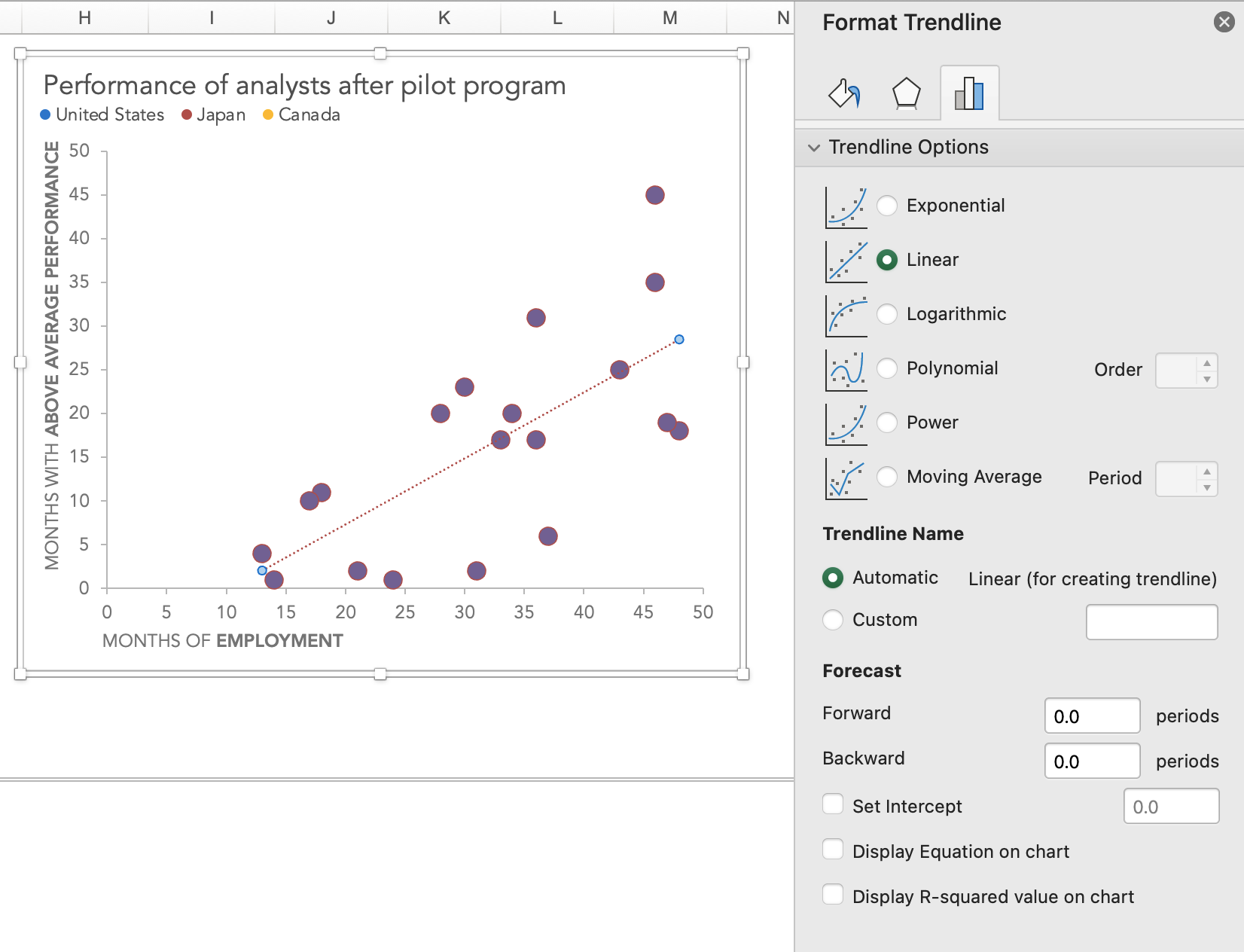
The red line in the view is the trendline Excel draws as its default option.
If you know what you’re doing with trendlines, here’s where you’d make your preferred adjustments; for our purposes today, all I’m going to do is mute the color of the line, and then turn off the fill and border settings for my “for creating trendline” data markers.

Using color, size, and line style to de-emphasize the default linear trendline.
How to add data labels to a scatter plot
It’s great that we’ve put our data on the graph…but what does that data actually represent? If we care about more than just the overall distribution of data points, we should add data labels to some, if not all, of our points.
To add data labels to a scatter plot, just right-click on any point in the data series you want to add labels to, and then select “Add Data Labels…” Excel will open up the “Format Data Labels” pane and apply its default settings, which are to show the current Y value as the label. (It will turn on “Show Leader Lines,” which I usually turn off.)
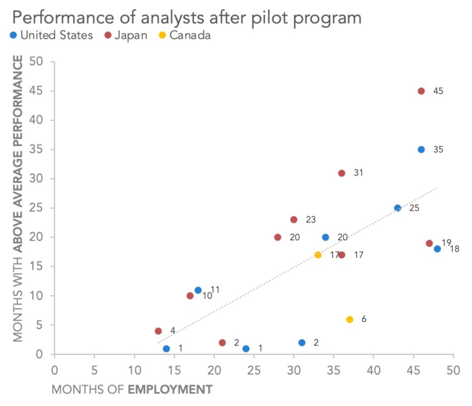
By default, Excel will add the Y values as the data label, and will align it to the right of each data point.
Using only the checkboxes in the “Format Data Labels” pane, you can get your labels to include other values or combinations of values, including the Series name, the X value, and/or the Y value. In many cases, though, we’ll want to customize our data labels to show other information than just those fields. For that, we’ll use the “Value From Cells” option.
How to customize labels in a scatter plot
You can tell Excel to use any cell or series of cells as its source for Data Label information. For instance, let’s label each of the markers in this chart with the first initial and last name of the pilot program participants. We can add a “Data Label” column to the right of the data table and use the CONCATENATE formula to create a cell in each row with this information.
You can use formulas to fill in your new “Date Label” column, or you can just manually add the data. In this version, we used the CONCATENATE formula to combine the first initial from the FIRST NAME column, a period, and the full LAST NAME column value for every row.
Then, click on a data label in the existing scatter plot. That brings up the “Format Data Labels” pane, where you can change the settings in the “Label Contains” section to use “Value From Cells”. Clicking on the “Select Range…” button brings up a popup window asking what cells to use for the data label information, and you can highlight all the cells in that brand-new column.

Select any specific range of cells to use as the source for your custom labels.
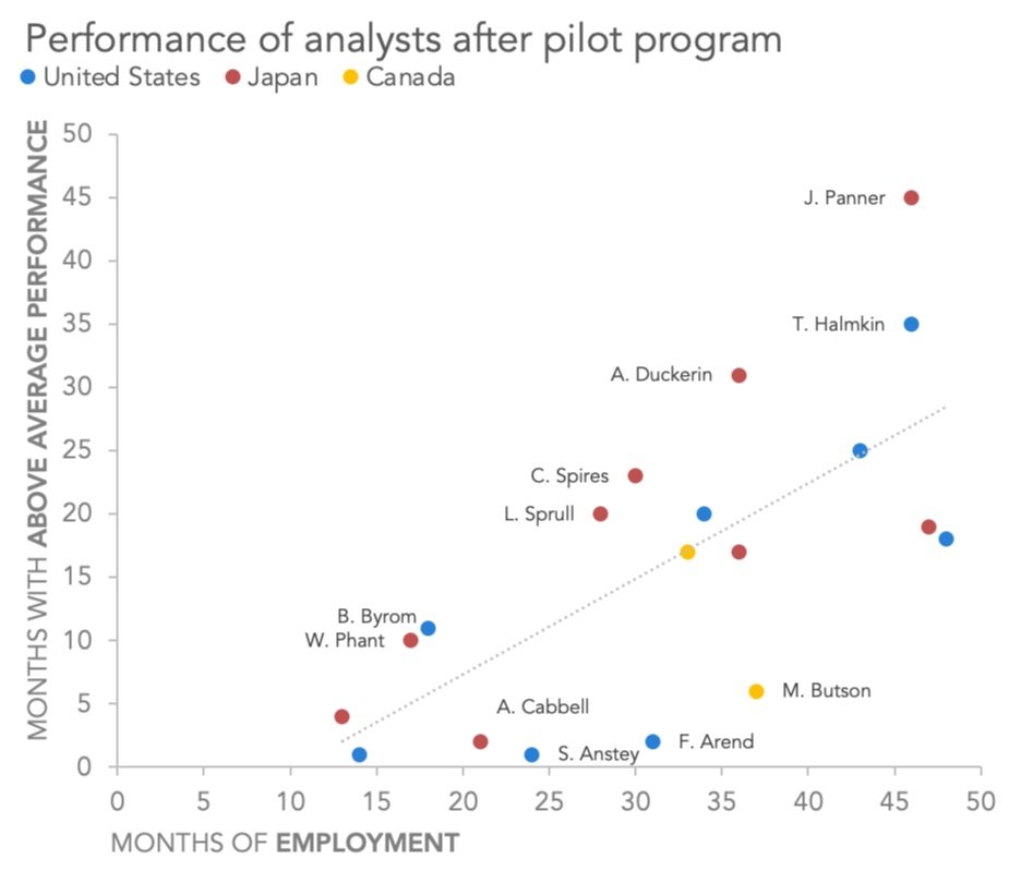
When you click OK, every data marker will be labeled..

All marks are now labeled with our custom values.
To reduce the amount of text in the graph, let’s only keep labels for those participants who were far above or far below the trendline—in other words, overachievers and underachievers.
Double-click on one of the labels you want to remove, and then either delete it or set its Text Fill to “No Fill.” Do the same to several other unwanted labels, until you’re left with just high- and low-performing participants. (You can also click-and-drag labels slightly out of their default positions, to make labels with close-by neighbors easier to read.)
Only high and low performers and lableled in this view.
How to put it all together
With the techniques described above, you should be well prepared to create a scatter plot in Excel that can be designed and formatted to support the specific story you intend to tell. Use the power pairing of color and words to help your audience see what you want them to notice and learn from your scatter plot. Feel free to include annotations inside or near the chart area itself, as well as large headline or takeaway text above your visualization to emphasize the key messages.

The final version of our visualization includes a takeaway title, annotations, a reference line, and custom labels on selected elements in our mult-series scatter plot.
Now, you’re ready to create your own scatter plots in Excel! The data and the graphs you see in this post (along with some bonus content) can be downloaded here.
Check out our chart guide for more about scatter plots and other graph types; subscribe to our YouTube channel for Excel tutorials and lots of other videos; and follow our blog to get the latest in how-to instructions, graph makeovers, and other tips and tricks for communicating more effectively with data.