what is a spider chart?
This article is part of our back-to-basics blog series called what is…?, where we’ll break down some common topics and questions posed to us. We’ve covered much of the content in previous posts, so this series allows us to bring together many disparate resources, creating a single source for your learning. We believe it’s important to take an occasional pulse on foundational knowledge, regardless of where you are in your learning journey. The success of many visualizations is dependent on a solid understanding of basic concepts. So whether you’re learning this for the first time, reading to reinforce core principles, or looking for resources to share with others—like our new comprehensive chart guide—please join us as we revisit and embrace the basics.
A spider chart, also sometimes called a radar chart, is often used when you want to display data across several unique dimensions. Although there are exceptions, these dimensions are usually quantitative, and typically range from zero to a maximum value. Each dimension’s range is normalized to one another, so that when we draw our spider chart, the length of a line from zero to a dimension’s maximum value will be the same for every dimension.
Spider charts can be found in lots of industries, but rarely in large numbers. In our experience, they’re most likely to pop up in food science (comparing products across multiple different facets of taste, texture, etc.) and in sports analytics (comparing athletes across several dimensions of performance). In one of our previous #SWDchallenges, several participants found other use cases for spider charts, such as comparing series on a time-cycle, comparing the volume of searches for different terms, or even visualizing the motifs in a piece of music.
How do you read a spider chart?
Just like line graphs, scatterplots, and many charts used in business communications, spider charts show data plotted on two different axes. However, the coordinate system that we use to plot data on a spider chart is a little less common: most business charts are drawn using Cartesian coordinates, but spider charts use polar coordinates.
Cartesian coordinates
Most common two-dimensional graphs, like scatterplots, use Cartesian coordinates—we use X and Y values to determine points’ locations on two perpendicular axes: the horizontal and the vertical, respectively.
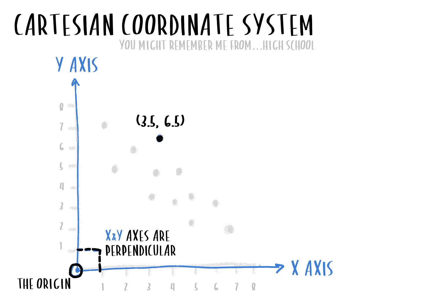
A Cartesian coordinate system plots data points along two perpendicular axes.
Each point gets a pair of values (the X and the Y), and we can look at the X/Y location of lots of points at the same time. In this way, we can get a good sense of the relationship between the X variable and the Y variable across every item in our data set.
Said more simply: this kind of graph and coordinate system is intended to aid the viewer in comparing two related measurements across several different items.
Polar coordinates
In a polar coordinate system, while we use two values to determine points’ locations, those values are “distance from the center of the circle” (or, “distance from the pole”), and “angle relative to a reference line.”
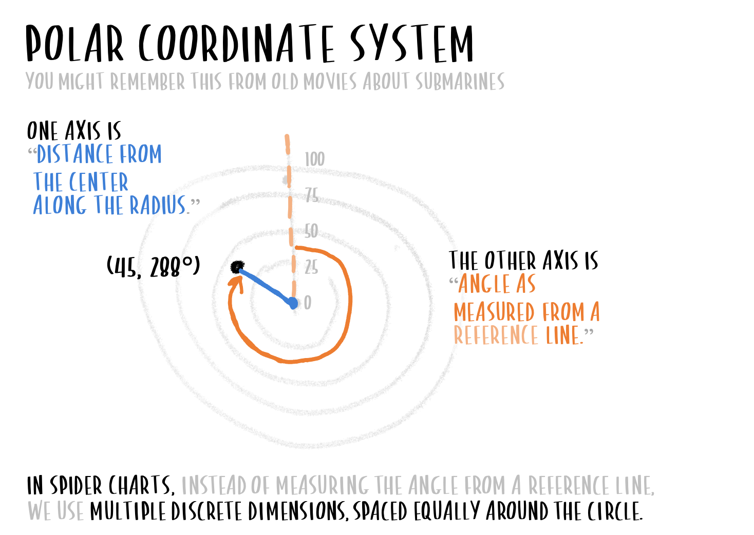
A polar coordinate system uses two axes as well: one axis radiating out from the center of the circle, and one axis defined by the size of the angle as measured from a reference line. In other words: one axis is linear, and one axis is radial.
For spider charts, our second axis (the orange one in the drawing above) isn’t continuous. Instead, we use a discrete number of fixed axes, each one representing a single dimension, spaced equally around the circle.
For spider charts, our second axis isn’t continuous. Instead, we use a discrete number of fixed axes, each one representing a single dimension, spaced equally around the circle.
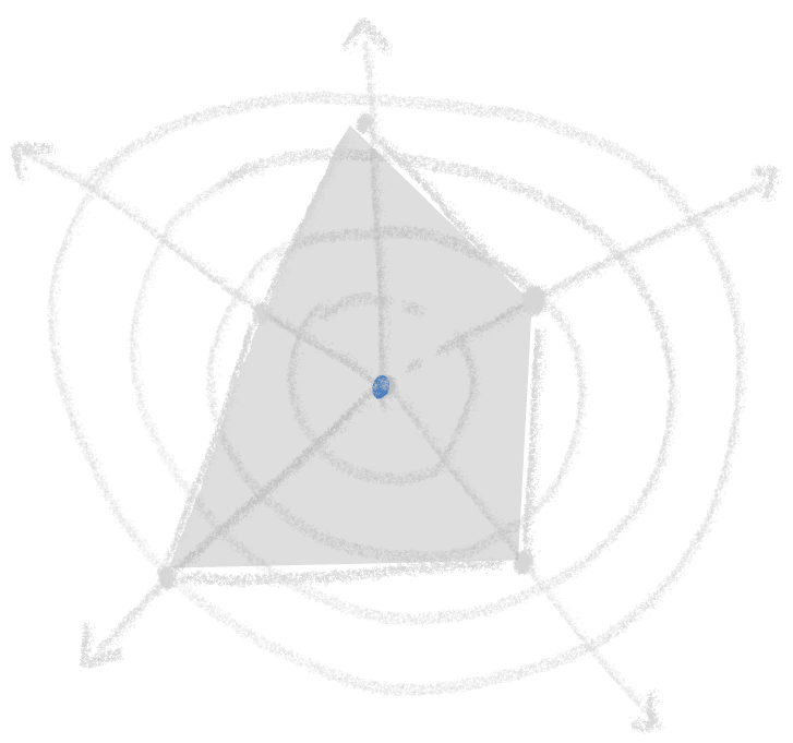
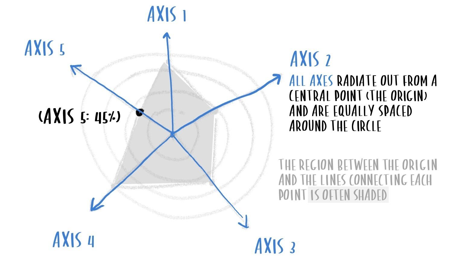
See how they kind of look like spokes coming out of the hub of a wheel? In a spider chart, each dimension gets its own spoke, and the spokes are evenly distributed around the wheel. The farther towards the end of the spike, the larger the value. Closest to the center means closer to zero.
With the freedom to use many linear axes, we could show lots of different dimensions for a single item simultaneously...but if we wanted to compare multiple items at the same time, we’d use several individual spider charts (in a small multiple format, perhaps). If it didn’t look too cluttered, we could also do a single overlay with multiple items stacked on top of each other.
This kind of graph, then, is best suited for comparing several different dimensions in a compact space, but for only one or a few items.
What’s the difference between a radar chart and a spider chart?
The terms “radar chart” and “spider chart” are used more or less interchangeably. It’s only logical to think that maybe we’d only call it a spider chart if we were going to connect the dots that we plot, to make the graph itself reminiscent of a spider’s web...but this is not the case. Whether they’re called radar or spider charts, the dots are almost always connected.
If several series are shown on the same plot, then the graph will start to look more and more like a spider web—especially if the designer chooses not to use color to fill in any areas of the graph. More often than not, the area between the chart’s origin and the lines connecting the dots is filled with a semi-transparent color.

The area contained by the connected dots in a spider chart is often filled in with a semi-transparent color.
On occasion you will also see alternating bands of concentric circles as fills. They’re meant to replace or augment gridlines, and help emphasize the size and shape of the filled area.
Also, depending on your tool of choice, your gridlines might be drawn as smooth circles, or they might be drawn as line segments connecting each successive dimension. The effect, then, is that instead of your gridlines being a series of concentric circles, they are a series of concentric polygons…as you’ll soon see in an example below.
When (and how) do I use spider charts effectively?
Spider charts are at their best when used to quickly compare multiple dimensions in a compact space. They can be attention-grabbing, due both to their circular structure and their relative novelty compared to other business graphs, so they can be effective when you need to visually engage your audience. A general audience might find them confusing or intimidating to read without additional guidance (which you can provide—we’ll talk more about that in a later section), but technical audiences might find them intriguing.
Let’s imagine that we have a classroom of students who all just took their final exam. For each student, we know a few different pieces of information:
Final exam grade
Midterm exam grade
Assignments completed during the term
Hours spent studying for the exam
Days absent (or, to make it more positive: number of classes attended)
Imagine then that we plot these values for one student, Arthur.
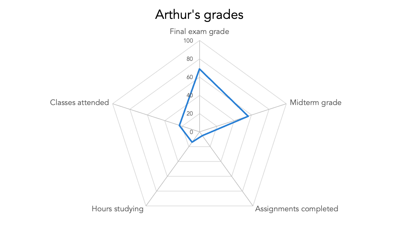
A spider chart plotting the raw data representing five dimensions of Arthur’s classroom performance.
Here you can see how my tool of choice, Excel, is drawing those gridlines in as polygons, rather than as circles. The data set for Arthur is plotted as a single line, connecting a series of points. Sometimes, you will see spider charts where the area contained by this closed line is filled in with a semi-transparent color.
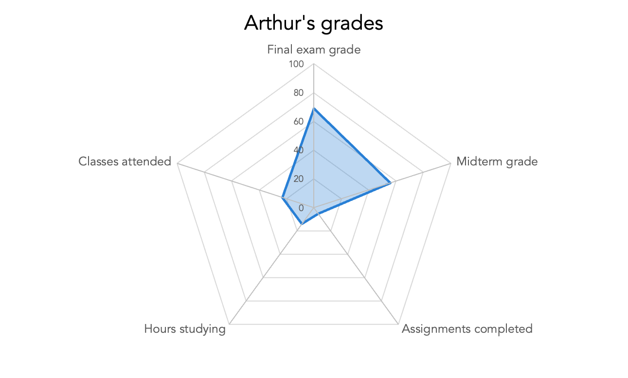
A spider chart plotting the raw data representing five dimensions of Arthur’s classroom performance, with the area circumscribed by his data points filled in with a semi-transparent color.
Because of the limitations of our tool, we’re using the same range (0-100) for each of these five dimensions. However, the domain is different for some of these measurements. For instance, there were only 25 class days and 12 total assignments, so it doesn’t make sense for those axes to go all the way up to 100.
One way around this limitation is to normalize the data. For each dimension, we know what value is the minimum possible value (zero), and which is the maximum possible value...or, if there is no limit to the maximum possible value (like, how many hours did you study for this test?), then we can use the maximum observed value within the class as the boundary of our domain.
When we normalize Arthur’s data—still using the actual values for our data labels—the spider chart now looks like this:
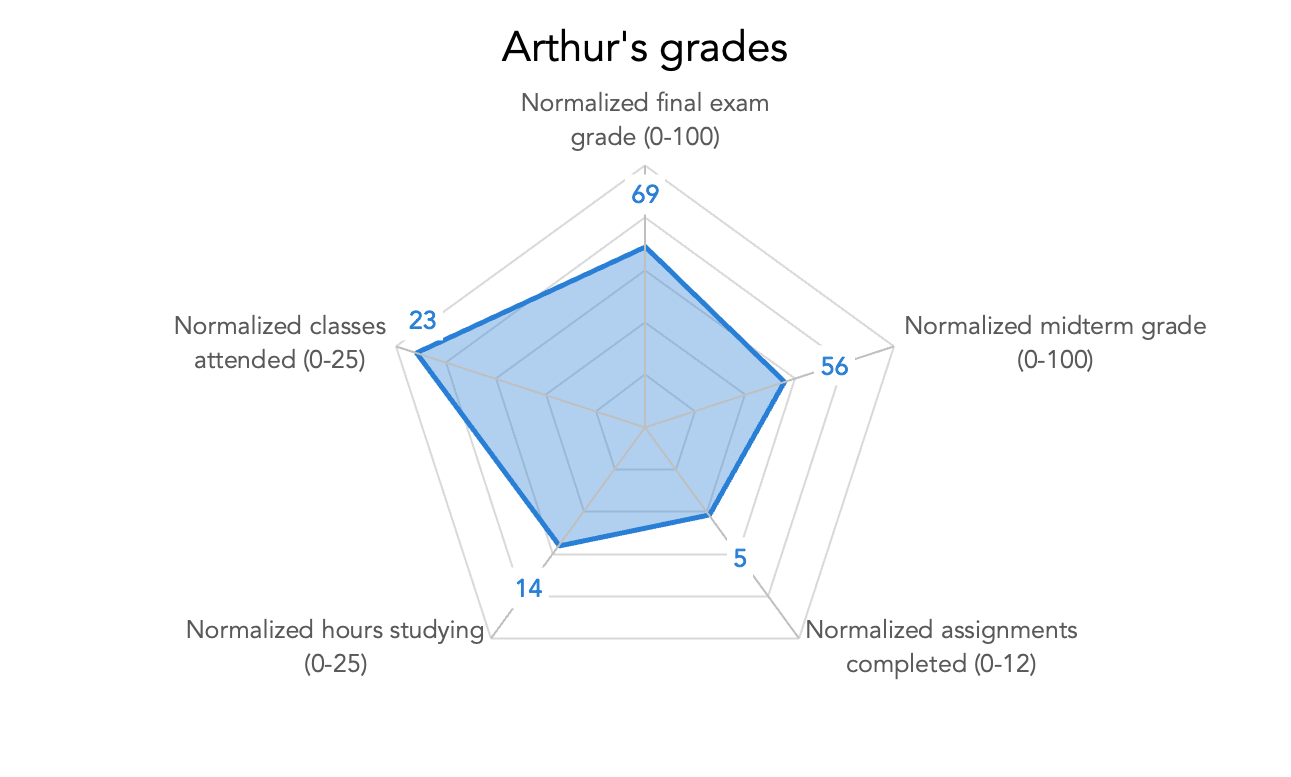
A shaded-in spider chart plotting the normalized data representing five dimensions of Arthur’s classroom performance. Each axis is now scaled from 0 at the center to the maximum possible value for that dimension at the edge.
It is possible that this is the view we want to use. We also might want to go a step further, and think about how Arthur performed compared to his classmates; that is, along each of these dimensions, into what percentile of actual results did he fall? By calculating the percentiles, we can then draw a spider chart where every axis’s range of values goes from 0 to 1, or from the lowest percentile to the highest. This will give us a better comparative view of the data.
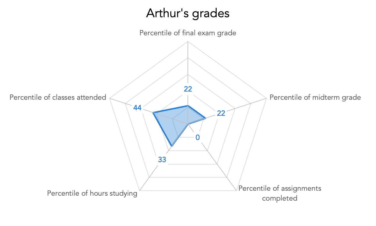
A shaded-in spider chart plotting the normalized data representing five dimensions of Arthur’s classroom performance. Each axis is now showing the percentile that Arthur fell into, within his classmates' scores, along each dimension.
When we applied this transformation to our data, Arthur’s chart got a lot smaller. It wasn’t clear before, because we didn’t have the context of the rest of his classmates’ performances, but Arthur seems to be one of the lowest-performing students. Let’s layer on two of his friends, Barb and Corey, for comparison.
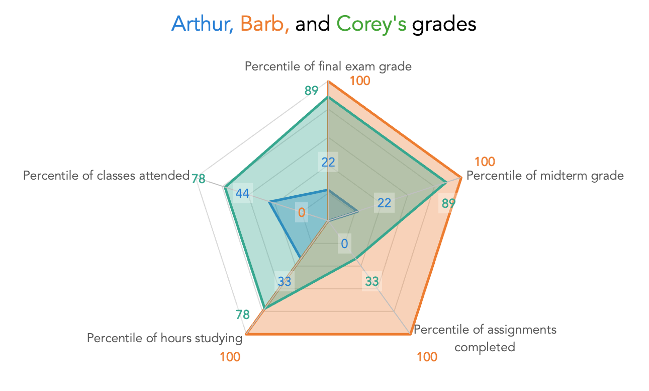
A shaded-in spider chart plotting the normalized data representing five dimensions of three classmates’ performance. Each axis is now showing the percentile that Arthur, Barb, and Corey fell into, within their classmates' scores, along each dimension.
With this context, we can make some visual assessments. Arthur didn't go to class as often as his classmates, did the fewest assignments, barely studied, and was near the bottom of the barrel on his midterm and his final. Barb was a superstar: she did all the assignments, studied hard, and aced both tests. The only knock against her as a student is that she missed class a lot, although it didn’t seem to hurt her performance. Corey, like Barb, succeeded on tests, but learned more from attending class than from doing assignments.
Things to keep in mind when you’re using a spider chart
Mitigate the challenge of comparing things by area
At the heart of it all, when we represent our data in a spider chart, we’re asking an audience to judge and assess that data by comparing areas. People are good at comparing data in one dimension at a time—bar charts are super easy to read—but are notoriously bad at comparing multiple dimensions simultaneously… even if it’s simple shapes like squares or circles. With spider charts, we’re asking an audience to compare the relative areas, angles, and peaks of irregular polygons (possibly while they are overlaid atop one another).
That already seems challenging, but there’s yet another layer of built-in complexity: our metrics for each chosen dimension will increase linearly along our radius. If we shade in the areas between the radius and the center of our plot, the area of that shading will increase geometrically, not linearly. That means that we will wind up visually overrepresenting larger values versus smaller values.
In a live setting, introduce your audience to this chart gradually
It will be helpful, in a live setting, if you can narrate and animate the building of your spider chart piece by piece. That way, this dense and potentially intimidating graph type could be introduced slowly and deliberately. By taking the time to escort your audience through the graph’s structure and meaning, you’ll be able to bring them to a complex and nuanced understanding of your analysis. If not in a live setting, you’ll likely have to annotate your charts liberally (or iterate to a simpler chart type to make sure the takeaways aren’t lost).
Order the axes thoughtfully and consistently
Since you could theoretically place the items in any order, the area that gets shaded in could have wildly different shapes and sizes depending on your choices. One way to mitigate this is to group meaningful metrics as close together as possible, and use the same order consistently every time you use a spider chart for all similarly-structured data sets. If your data lends itself to grouping or to supercategories, you could use color to help your audience visually distinguish among them.
Consider similar alternatives
A parallel coordinates chart is somewhat like an unspooled spider chart. Instead of each axis starting from the same point of origin and radiating out from one another, we place those axes in parallel, vertically. Then we end up comparing things on the Y axis, as each one of our metrics is one spike along the X axis.

This parallel coordinates chart is based on the same data that we used in our spider charts, but by “unwinding” the chart into a straight line, it can make the comparisons across students easier to see.
It’s not as elegant as a spider chart visually, but it can make the comparisons easier to see, as it resembles the far more common line graph and as such will feel more familiar to a broader audience. One downside, however, is that it isn’t, in fact, a common line graph (each vertical axis is a different scale), and its resemblance to one may lead to a casual viewer misinterpreting the visual entirely.
Final thoughts
Spider charts can be appealingly efficient, because they can visually encode a lot of different information in a small area. Keep in mind, though, that an unfamiliar audience may need to expend a lot of effort in order to read them, or to understand a key takeaway. When a spider chart is essential to communicate something specific, make sure you’re supporting your audience’s understanding through narration or step-by-step animation. If that isn’t an option, then consider using a different, simpler chart to make your insights clear.
To learn more about other charts, browse the full collection in the SWD Chart Guide, or for resources to teach younger audiences, check out DaphneDrawsData.com.
Master complex charts in our NEW! on-demand learning course
Learn in-depth techniques for creating, designing, and effectively presenting more novel views in PowerPoint. Through step-by-step video lessons, you'll master radar charts, box plots, scatterplots, horizon charts, and bubble graphs. With optional exercises to reinforce your learning and bonus materials covering additional graph types, this course will elevate your data presentation skills. Enroll today!