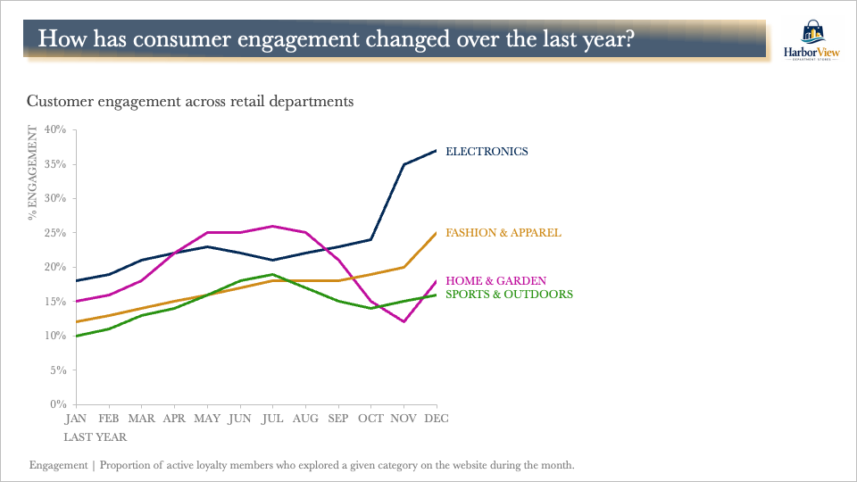
use color to focus or to compete for attention

Getting your audience’s attention and focusing it well are critical components of building a successful data communication. While there are several ways to capture attention, the two techniques we find most effective—and the ones we talk about the most—are: 

1. employ words more thoughtfully, and more liberally, in support of our graphs; and

2. apply color more sparingly but intentionally to make the important elements of your visual stand out.

However, the context in which our messages are presented dramatically influences the amount of attention we need to compete for. As you can imagine, there’s a huge difference between  presenting a detailed slide deck to a small, engaged group and sharing visuals on social media in the hopes of capturing the fleeting attention of millions. We can use words and color to focus attention in both scenarios, but our tactics and our goals will vary tremendously.

---

As a case study, let’s use a recent investigation on the Rolling Stone “500 Greatest Albums of All Time” list, Chris Dalla Riva, a musician who does a great deal of data-oriented writing about music, co-authored a piece with Matt Daniels of the Pudding about the differences between the version of the list from 2003 vs. the version compiled in 2020. The whole piece is worth a look for any music fan, but one facet of the analysis I found interesting was the composition of the voter pool for the different lists. 

Working on the assumption that the music we all have the strongest affinity for is “whatever was popular in our teen years,” Dalla Riva and Daniels could have created a simple paired bar chart to show how the “teen years” have shifted between the two voting cohorts.

A simple paired bar chart like this could have communicated how 2003 voters’ teenage years were mostly in the 1980s or earlier, while more than half of the 2020 judges’ teenage years were in the 1990s or later.

While this would have been an accurate accounting of the data (the 2020 list has much younger voters in it, while the 2003 list was created mostly by Boomers and Gen Xers), and it might have worked in a business PowerPoint, it wouldn’t have moved the needle very much in terms of social media engagement.

Even in a business setting, I might have suggested that a paired bar chart could be improved upon. Another option would be to use a simple diverging bar chart, sorted by the decade of each voter’s teenage experience, to show one potential cause of the lists’ differences.

With words and color now doing a bit of work here, the diverging bar chart represents the story slightly more effectively. Look how we’re using data labels selectively, putting our annotations on the page and close to the data, and keeping our colors uniform across text, legend, and chart. It’s an improvement, but it’s got a ways to go to be a “scroll-stopping” image.

Accounting for this chart being part of a larger story (one that delves more deeply into the albums on each list, not just the judges behind the decisions), and that story utilizing a dramatic “dark mode” color palette, another option could have been to keep that diverging bar chart, but with a fresh coat of neon paint:

Now we’re talking. With a less common but still highly contrasting color palette, a dramatic dark background, some fading out of less-important data points, and the addition of context (the total judges for each list), this is beginning to feel like a visual that could be the accompanying image for the full article…or could it?

Considering how “creative” we often get in our day-to-day PowerPoints, the above version of the chart feels good. In the context of the office, it’s likely all you’ll need. Dalla Riva and Daniels, however, know that they have an astoundingly more difficult task that we often do in terms of competing for their audience’s attention.  

Instead of getting to a simple diverging bar chart and calling it a day, they crafted something far more memorable, engaging, and useful. In a choice that aesthetically and thematically carried through all of the visuals in their story, they used thumbnail images of the voters themselves to build the bars—a choice that made the design more distinctive, compelling, and conducive to both granular exploration and high-level summary assessment.

This screenshot of Dalla Riva and Daniels’s actual design, using thumbnails of judges’ portraits to denote when their individual teenage years were, barely does it justice. 

Moreover, those thumbnail photos animate as you scroll through the story, dimming and flying to different visual configurations as the voter cadres are depicted by actual age, gender, and other meaningful cohort differences. I strongly encourage folks to explore the interactive themselves to get the full experience.

It’s undeniably fun to explore and experiment with color and design. Usually, for business communications, they’re best deployed to bring people to that most granular level of focus and understanding. In a different context, though, where your audience has a much lower level of initial engagement, you may find yourself needing to use the power of color very differently, just to break through the noise and get your communication noticed at all.

from touchdowns to takeaways: a Super Bowl commercials makeover

More than 100 million people tuned in to watch the Kansas City Chiefs defeat the San Francisco 49ers in last weekend’s Super Bowl, which has evolved beyond a mere sporting match to something more like an unofficial American holiday. Historically, while many tune in for the football itself, a significant number of viewers are equally interested in the commercials. The team at SWD tracks along with both the football and the advertisements, but also a third aspect: any data visualizations associated with the game.

As a case in point, our friend and former colleague Elizabeth shared a graph with us that she discovered in an article published in the run-up to the game. We’ve recreated it below; it illustrates the most common Super Bowl commercials by industry over the last five years, providing a glimpse into a tradition that spans even further. 

The bold palette of this graph is certainly a scroll-stopper, which is a necessity when competing for attention in a week saturated with Super Bowl content. This rainbow color scheme does an excellent job of catching the eye.

However, as I scrutinize this chart through the lens of a data storyteller, I naturally start to think about the intent behind its creation. What are we meant to discern from this visualization?

A useful principle to remember is that the most straightforward comparison—that is to say, the easiest comparison to make visually—often reflects the creator's intended focus. In this instance, each year is represented by a different color in a stacked bar, and each commercial category has its own bar.  

Since the easiest thing to do here, visually, is to scan across the tops of each stack of bars and compare their heights against each other, my assumption is that the graph was created primarily so we could see which categories had the most advertisers over the past five Super Bowls.

The categories are sorted alphabetically (with Wellness & Insurance as the notable exception…if I had to guess, I’d suggest that the category was originally called Insurance & Wellness but was re-named at some point in the process without also being re-sorted). This arrangement is useful for long lists of categories, if the goal is to make it easy for someone to find a specific category quickly. However, if the aim is to highlight which categories are most and least prevalent, a more logical approach would be to sort them from most to least.

While the categories are now sorted meaningfully, the visual is still harder to interpret than it needs to be, owing to the diagonally placed category labels. Rotating this vertical bar chart to a horizontal bar orientation would allow the labels to be written in a single, easily readable line.

This adjustment makes the graph more navigable and the category names clearer, yet the vibrant color scheme still dominates the view. Now I have to wonder if the rainbow palette has gone past “attention grabbing” and into “overly distracting.”

Let’s think back to answering the question of the purpose of the visual. 

• If the goal is to observe the fluctuation of commercials across categories over the five years, we could better achieve that by iterating to a different graph type. (Foreshadowing!)

• On the other hand, if we’re meant simply to compare the overall category trends, toning down the color usage might be beneficial.

I may start by making every year an identical gray color…

…and then perhaps bring some color back in, just to highlight selected aspects of the data. Maybe we could color in only the year with the highest number of commercials in each category? 

Ugh, no. This results in a visually chaotic and demanding graph. If you can stand to look at it long enough, this view reveals some interesting trends, like the predominance of entertainment and alcohol commercials in 2023 and the beginnings of sports betting ads in 2022. More importantly, though, it underscores the need for a clearer visualization method for depicting changes over time.

Whenever I hear the phrase “over time” in my head in relation to data visualization, it’s a cue for me to at least try a line graph. For showing continuous data such as we have here, it seemed a promising alternative. 

Unfortunately, as is painfully obvious here, a standard line graph quickly proved unsuitable with this data set. It wound up looking like a "spaghetti graph"—an overly complex visualization with numerous overlapping data series. 

There are alternatives, however, when faced with this situation. Small multiple charts, which break down the data into individual series for easier comparison, offer a cleaner, more comprehensible format.

This visualization type allows us to create a grid of smaller, identically-scaled versions of the same axes for each data series independently. Scanning across all of them makes it easier to pick out variations in trends, peaks, valleys, and other anomalies. While they could be sorted alphabetically, here they are sorted from left to right, top to bottom, in order of total number of commercials across all five years of data.

Adopting small multiple charts for line graphs clarified the trends—we can see the dominance of Food & Beverage, the one-year peak of Entertainment in 2023, the rise and fall of Fintech—but makes it more challenging to see the volume of advertisements.

More so than line graphs, bar charts imply that the data they represent can be counted, or measured. Line graphs are excellent choices for showing rates, ratios, position on an arbitrary scale (like temperature)—anything where there’s not necessarily a meaningful relationship to zero. Bar charts, on the other hand, by their visual nature, imply that there is an amount of something. If one bar is twice as big as the next one, we think that there’s twice as much of whatever it is we’re graphing. Conversely, 100 degrees isn’t “twice as hot” as 50 degrees. 

The number of commercial advertisers in each category, in each year, is a countable, measurable value. If we use bar charts instead of line graphs, we can intentionally emphasize that aspect of our data. 

This bar chart version of a small multiple graph presents a more intuitive representation of volume, but now the trend is more challenging to see, since there’s now a "stair-step" effect to the change over time.

At this point, I’m torn. I appreciate aspects of both line graphs and bar charts here, but each one seems to be a little bit lacking. Ultimately, I found myself drawn to a graph I rarely reach for: the area graph. In most cases I find them too easy to misinterpret, and often overly complex. However, in a small multiple format, this approach effectively balances the visualization of trends over time with the representation of volume, fulfilling both objectives without overwhelming the viewer.

If tasked with sharing a visualization of this on social media, I would likely opt for the area graph small multiple chart. It maintains visual interest while facilitating more straightforward comparisons across categories over several years. Although the colors used do not carry inherent meaning, this compromise is often necessary when engaging a general audience, as opposed to the more focused use of color in business communications.

---

As we’ve iterated through various visual formats, we’ve also explored our data from a few different perspectives. This has yielded insightful observations, particularly regarding the dominance of the Food & Beverage category in Super Bowl commercials, with notable fluctuations over the years and a brief overtaking by the entertainment category in 2023. We also noted that the Fintech category also displayed interesting peaks in 2021 and 2022, particularly influenced by cryptocurrency and mortgage broker ads, which vanished by 2024.

In a business context, with a captive audience more interested in key takeaways, I would likely discard the small multiple view entirely. Instead, I’d employ a combination of line graphs with descriptive captions to convey these insights more clearly.

Ultimately, there is no singularly correct approach to data visualization. The key is to consider the audience's needs, the context of the presentation, and the intended message. Visualizing data is as much an art as it is a science, requiring experimentation, iteration, and feedback, rather than adherence to a strict set of rules.

Just as teams like the Kansas City Chiefs demonstrate through their repeated victories and strategic gameplay, excellence in data storytelling also requires continuous practice, experimentation, and adaptation. Each attempt at visualizing data—whether through bar graphs, line charts, or small multiples—serves as a learning opportunity, guiding us towards clearer, more impactful communication. 

challenges with double donuts

Recently, I’ve gotten a couple of questions about donut charts: Are donuts a good alternative to pies? When would you use a donut chart? Food-wise, I’d be happy for either a pie or a donut—both are great! However, graph-wise, I find both can be challenging. We’ve posted about pie charts before and explored some alternatives to pies. A donut chart is a cousin to the pie chart—it's essentially a pie chart with a circle cutout in the center. It turns out that the same limitations of pies also apply to donut charts.

Let’s consider the real-world example below.

Here we have not one, but two donuts! It takes a while to figure out what this data represents. Based on the title, it appears that we’re meant to compare the categories of the donuts across the two charts. With the sections in different places, this is rather challenging. 

One may argue that the colors and donut form make the data more visually interesting; however, this often hinders our ability to understand the data. Let’s look at some strategies to make this information easier to comprehend.

Order data in a thoughtful and intuitive way

Starting at the top of the donuts and working clockwise around, the categories are arranged in alphabetical order. This order works well if someone is looking for a specific category and wants to quickly look it up in the list (particularly a long one). In this case, however, it may be more interesting to quickly scan to see the highest and lowest project risk categories. By plotting the values in both graphs in order from most to least Issues Raised, we can make this task simpler for our audience. 

Now we can see the Supplier, Schedule, and Budget categories are the top three in Issues Raised. We can also start to see some differences between the two visuals. For example, Supplier is not the top category for Issues Resolved in the right graph.

Put things you want to compare close together

Having physical distance between things makes comparing them more difficult. Other chart types, like bar graphs or slopegraphs, would allow us to put the categories next to each other for an easy visual comparison. Since the Issues Resolved are a subset of the total Issues Raised, I’ll opt for a stacked bar chart using absolute values, instead of percentages.

Having the information on a common axis now makes the task of comparing the categories and the status of the issues much easier.

Apply colors sparingly and use words wisely to make the takeaway clear

Using stacked bars with just two categories—Resolved and Unresolved—also helps to reduce the number of colors that were in the original donut charts. Rather than applying color for decoration or interest, or to make multiple categorical distinctions, we should use color sparingly and strategically to draw our audience’s attention to what we want them to see. We can also make the point of the visual clear by writing out the takeaway and including it next to the data. This helps people know where to look for the evidence of what you're telling them.

Check out the impact of simplifying the original view to make less work for our audience to understand and see the main takeaway.

Note that there is a time and place for donuts (and pies!)—see our related challenge for some ideas if you are considering one of these circular-shaped charts.

---

Do you want to learn to create and communicate a powerful data story? Join our upcoming 8-week online course: plan, create, and deliver your data story. Data storytellers Amy and Simon will guide you through the world of storytelling with data, teaching a repeatable process to plan in helpful ways, distill critical components, create effective materials (graphs, slides, and presentations), and communicate it all in a way that gets your audience’s attention and drives action. Learn more and register today.

when simple charts are surprisingly confusing

Here's a tip we share frequently: keep your charts as simple as you can. Limit the amount of information you display at any one time, use graph types people know, and explain with clear, precise words what the visual is showing. These steps go a long way towards making your message easy for anyone to understand.

With that in mind, it's hard to believe that a simple bar chart with a single series of data could ever be considered to be confusing. But making a chart truly simple starts way before you make any design or graphing decisions. 

Recently, I was working with a company that helps small local businesses understand their sales and consumer data. One of their clients, a coffee house called Mellow Bean, receives regular updates and analyses on both their own sales and their competitors’ sales.

As part of my collaboration with them, the company shared a graph with me from Mellow Bean’s monthly report. Before going into details, let’s look at the chart. If a picture is worth a thousand words, it should speak for itself, right?

Looking at the chart, you might think, “For such a simple chart, why am I so confused?” It's a bar chart with one data series, a title, a subtitle, and more info at the bottom. But the real challenge isn't the design, layout, or labeling. It's the assumptions made before creating the chart. For example, the chart uses the acronym "ADS" without explaining it. Does everyone know it means Average Daily Sales? And does “Gap Analysis” make sense to coffee shop owners?

Let’s take a two-stage approach to strengthen this graph. First, without changing the underlying visual much, if at all, we can use words to make the key messages easier to understand. Second, assuming we have the time, inclination, and authority to modify the graph itself, we can iterate to a visual that more neatly dovetails with the newly-added text.

FIRST STAGE: improve the text 

The average viewer seeing this visual will have to do a bit of detective work to fully understand it. They’ll have to look at the text above and below the chart, guess what "ADS" means, and figure out why the dollar amounts in the graph are so small. (It’s probably because they're averages, not totals; my condolences to the coffee shop with $20 in monthly sales!)

Now let’s clarify things. I’ll restructure the text surrounding the graph, by both highlighting the main takeaway at the top and labeling the bars more clearly.

We’ve now made it easier for viewers to understand what's happening, but there is still more we can do. Adding some context, like the fact that September sales went up due to students returning to the university campus, will give a fuller picture. Mentioning the exact ADS for Mellow Bean, and how big the gap is between top competitors, also helps.

We can improve further by suggesting what to do with this information. What action should Mellow Bean take based on this data? Let’s add that in as well.

SECOND STAGE: improve the visual

Once we've cleared up the message with words, we can think about how to visualize it better. Instead of just showing gaps, why not display the actual Average Daily Sales for each competitor? This gives a clearer sense of the revenue differences between the coffee shops.

What’s easier to see, once we’ve switched to this new bar graph?

• Pore Over, the obvious outlier, is in a class by itself.

• Mellow Bean is close to, but trailing, two competitors with similar sales levels. 

• Below Mellow Bean, the next two cafés are about $150–$175 behind on daily sales.  

Even though all of this information was explicitly visualized in the original graph, it doesn't feel intuitive the way that it does when experienced in this more commonly seen layout.

We could go a step further and include these explicit gaps as well, simply by adding a smaller bar graph to our new design:

Let’s quickly compare where we started and where we are now:

With these changes, the chart becomes more accessible and easier to understand for everyone. Even though both graphs use text to add context for the viewer, the graph on the right uses full sentences, complete thoughts, and more intentional labeling, color, and position of that text, all of which leads a viewer to a more robust understanding of the scenario and an idea of what to do with that information going forward.

Keeping things simple isn't just about choosing common charts, adding a few words of context and minimizing the amount of data you show. It’s essential to take a beat, consider the audience’s perspective, and imagine how they’ll feel when they first see the communication you’re planning. If you skip this thoughtful consideration up front, your audience may well discover that even a simple chart can end up being surprisingly confusing.

better than a big bar chart

Maybe this has happened to you: you’ve been presented with either a super wide or super tall bar chart that compares two different data series across dozens of categories.

You try to make sense of the comparisons across the entire graph…but with so many bars of alternating colors, it looks less like a data visualization and more like a test pattern, or an old-school 3-D image that you can’t see without those red-and-blue glasses.

Let’s take a closer look at that extra-tall bar chart. I came across a graph like this one when working with a recent client. They created a visual to compare the quarterly sales revenues for each of 25 different sales associates against their individual sales targets.

I took two different approaches to strengthening this graph: the first one keeps the same chart type but uses more approachable design choices; the other leverages a less-common but powerful visual, specifically well-suited to making these pairwise comparisons easy to see.

Option 1: Fill the thermometer

The first option for improving this view stays within the bar graph family. Instead of pairing bars and asking an audience to try to keep track of those alternating data series, I took inspiration from traditional fundraising posters. As they encourage prospective donors to “fill the thermometer” in order to meet a revenue goal, I also created thermometers to represent our Revenue Targets series. Instead of teal, solid-filled bars, I changed them to be outlined but unfilled. 

Then, I filled the thermometers with the actual sales revenue each associate generated in Q2:

Aside from the obvious improvement in aesthetics we gain by discarding the garish red and teal, we also benefit by getting more vertical breathing room for each row of data, since each associate’s two bars are now overlapping one another. 

This is a good solution when most or all of the actual data is below the target value, but it’s still a challenge to see which, if any, sales associates exceeded their targets. In fact, eight of the 25 did, so we could also use different intensities of blue in our Closed Deals data series to highlight those overachievers.

As much as I like this visual metaphor of filling a thermometer, we can also use a different option that isn’t quite so ink-heavy.

Option 2: Connect the dots

If we don’t restrict ourselves to just using bar charts, we can use an even better way to highlight these comparisons. By implementing a slightly different graph type, we remove a lot of extra visual clutter, lighten up the view for an audience, and give ourselves the chance to add in thoughtful labels and annotations. The graph type I’m talking about is a connected (Cleveland) dot plot.

You could think of this visual as a variation on the “fill the thermometer” chart, except that instead of drawing full bars, you’d simply put data markers where the ends of the bars would be, as I did here:

Here, I chose to represent the target value as an open circle, and the actual sales as a filled blue circle. Sometimes (as in this example) you’ll see lines connecting the two dots—charts like these are sometimes called barbell graphs. If there are multiple dots per row, a line may connect the dot with the largest value to one with the smallest in order to make the full range for that row easier to see. 

Since this view is sorted in descending order of sales target, there’s a visually appealing diagonal spine that runs down the center of our chart. From that spine, little lollipops pop out to the left (if the associate didn’t make their target) or to the right (if they did). The directionality of the solid marker, in contrast to the open Revenue Target marker, helps to show who made or missed their goals. My personal feeling is that more emphasis is needed, so I made more intentional use of color to make that message explicit.

At a glance now we can tell that anyone whose name is in orange, and whose marker is in orange, failed to meet their sales target. (The color of the barbell itself could also be changed to match the marker, but I chose to forego that just as a personal preference.)

When I was working on these visuals, I was not sure what relationship in the data my client cared most about. Did they want to highlight top revenue generators? Celebrate overachievers? Call out the people who missed the mark by the greatest amount? Our sort order would change depending on what point of emphasis they wanted.

For example, re-sorting based on the greatest difference between target and actual sales created a less elegant-looking graph, but one that drew attention to the associates who went above and beyond expectations.

Eventually I settled on a sort order that prioritized the amount of revenue each associate brought in, regardless of their target:

Having decided on a graph type, color choices, and a sort order, it was time for some finishing touches. There are a couple of inherent challenges with connected dot plots: the reliance on gridlines to connect the data labels to the data markers, and the distance your eyes have to travel to connect those labels and markers at all.

I do like the consistent alignment of the associates’ names along the vertical axis, but in the end I thought it was more important to bring the labels and the data markers closer together. I chose to align the names either to the left or to the right of the Closed Deals markers, depending on whether the associate beat the sales target. (I also included the actual sales amount in the data label.) This allowed me to get rid of the gridlines entirely and gain a bit more horizontal space for my plot area.

Dot plots are woefully underused in most business communications, and I have my suspicions as to why. Although you can create them in just about any tool, connected dot plots are not available as default graph types in Excel, PowerPoint, Power BI, Tableau, Qlik, Domo, Looker Studio, or MicroStrategy. (They are, however, in basic libraries for R and Python, and are easily created with online tools such as flourish.studio and Datawrapper.)  Even so, it is fairly easy to find step-by-step instructions online for creating these charts in your tool of choice. 

Whether you would prefer to stick with the “fill the thermometer” style bar chart, or are motivated to give connected dot plots a try, either option is an aesthetic and substantive improvement over the endless alternating bar chart. Your audience will thank you for it.

declutter a dual y-axis chart

Have you ever felt overwhelmed when you open an overflowing, unorganized closet or enter a crowded room? It’s a common reaction when you receive too much visual input at once. We often experience this same uncomfortable feeling when presented with too much information in a graph.

Consider the following dual y-axis chart and take note of how it makes you feel.

An example dual y-axis chart—also referred to as a combination or secondary axis graph.

You may be confused and overwhelmed at first. Dual-axis graphs like this are inherently challenging. Whether you call them dual-axis graphs, combo charts, or secondary y-axis graphs, they always demand extra effort from a reader to figure out which data series to read against which vertical axis. 

Explore dual y-axis alternatives

 We can eliminate this effort by using one of two alternative approaches:

1. hide the vertical y-axes and instead label the data directly, or

2. pull the graphs apart vertically so you can still leverage the same x-axis across both, but each gets its own left-hand y-axis.

For this example, the second option—separating the charts—is a better approach since the lines are overprinting on the bars.

An alternative to a dual y-axis chart: separate and stack vertically.

Now there are two separate graphs, but they are organized so they still look like a single visual, and the horizontal axis can be read across both. Since they each have their own y-axis on the left-hand side, there’s no more confusion about which scale goes with which data series.

This is a better view than the original chart, but there is more we can do here to make the graph easier to read and understand.

Eliminate non-essential elements

By default, our graphing tool—Excel in this case—has included gridlines and extra decimals. Stripping away these elements that are taking up space but adding zero information value will simplify our visual and allow the data to stand out further. At the same time, let’s add y-axis titles and tick marks to make things more straightforward for the audience.

Removing gridlines and providing clear vertical axis titles along with tick marks for reference make a more clear graph.

Consider how much data is required

We could make the visual easier to digest by plotting less data. For instance, we may not need so much historical data presented on the horizontal axis. Are subscription prices for every quarter in 2019, 2020, and 2021 necessary here? Let’s assume that for our purposes, only the previous year’s (2022) and current year’s (2023) data, along with next year’s (2024) projections are pertinent. Displaying only the relevant data reduces the cognitive effort required to understand the information.

Let’s also take the opportunity to remove the repeating year labels by using super categories, gaining space to rotate the x-axis labels horizontally, making them easier and faster to read.

Show the appropriate amount of historical data—here we are only displaying last year, this year, and next year’s data.

Iterate to a more appropriate chart type

A different chart type could make things easier for our audience. By swapping the profit bars for a line, we go from twelve dense and heavy bars to one simple line, which provides more space to add additional context and annotations for the viewers of the graph. Line graphs also enable us to zoom in on the vertical axis since we no longer need to show the full values of the bars.

Finally, let’s remove the bottom legend since the axis titles clarify what each series represents. (If we were plotting multiple series against each axes, we could label the lines directly instead.)

Consider lines instead of bars for time series data.

Clearly title the graph

So far, we’ve talked mostly about what we can remove from graphs for clarity’s sake. We also want to be thoughtful about including necessary details so our audience understands what they are looking at. Crafting a clear chart title helps them avoid confusion and faulty assumptions. While adjusting the title, switching from title case to sentence case makes it faster to read and left-aligning the text creates a nice framing for the graph.

A title cased and left-aligned chart title is easier to read.

Differentiate forecast from actual

Our graph includes future data: the remainder of this year (Q3 and Q4 2023) and next year’s (2024) data. This information represents a forecast of what is expected to happen. This should be clearly differentiated from actual data so people looking at the chart do not come to the wrong conclusion. Using dotted lines, a vertical reference line, or a shaded region like below are effective approaches.

A shaded region can help to differentiate actual from projected data.

Focus attention

Now our graph is much simpler and clearer than the original dual-axis view, but you may be left wondering why you are looking at this information. We can go further and add details to make our point evident to our audience. With sparing use of color, words, and other design choices, we can show where to look and make the main takeaway clear. 

Use words and color sparing to make the main takeaway obvious.

Minor changes have a major impact

Check out the impact of our deliberate steps to simplify the original dual y-axis graph. Each change by itself was relatively minor, but when applied together the final view is less overwhelming and easier to understand. 

Intentional design steps to declutter and focus are proven to be clearer and more credible while increasing recall. For more practice, watch our step-by-step Excel declutter video and tackle a decluttering exercise.