supercategory axis labels in Excel

I have a super quick tip to share today for those reading who work in Excel. I see graphs regularly that look similar to the following:

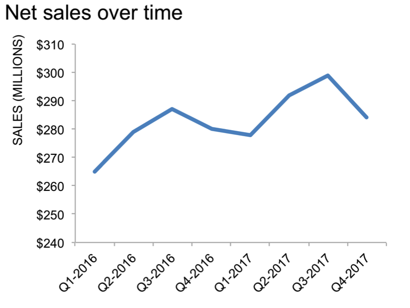
Note the x-axis. It isn't awful. But it also isn't ideal. The years are repeated. It looks a little sloppy. "Lack of attention to detail here? What does that mean for all the steps behind the scenes that I can't see?" your audience may be wondering. Also, studies have shown that diagonal text is about 50% slower to read than horizontal text. So if efficiency of information transfer is one of your goals when communicating with data—which I would argue it should be—aim for horizontal text whenever possible.

In Excel, there is a quick trick to fix this. I get asked how to do this regularly, so figured it warrants a quick "how to" post. I'll focus on the x-axis using the above example—you could follow a similar process to create supercategory axis labels on the y-axis when that makes sense, too. Also, this example uses quarterly data but you could follow the same process with monthly data.

In the Excel spreadsheet, the data graphed above looks like this:

The current x-axis labels (DATE) are in the column on the left and the y-axis values (SALES) are in the column on the right. Start by highlighting these and creating your graph. It will look similar to the graph at the beginning of this post.

Next, we need to add a couple more columns of data to split out the year and quarter (the process would look very similar if you have monthly data). I typically add two columns to the left of my original data to do this (new columns highlighted in blue):

Once you've done that, right-click on your graph and go to "Select Data."

In the menu that comes up, "Category (X) axis labels" (highlighted in blue at right, below) will be pointed at the original DATE column (mine, as you see below, was in Column D):

Click on this and use your mouse to highlight the range of both of the new columns you've added (my YEAR and QUARTER data was in columns B and C, respectively).

Hit OK, and your graph will look something like this:

Voila! A beautifully formatted x-axis. If it would be helpful, you can download the Excel file.

Would it be helpful to see more Excel "how to" posts like this? Let me know if there are specific topics or questions of interest that we can answer here by leaving a comment. Do you have any quick tool tips you'd like to share (Excel or otherwise)? Leave a comment to enlighten us all!